Table of contents > Defining viewer nodes
Of course, we could just print the output of our get_circle node from the previous chapter using the print() node. However, since we may find ourselves working with more complex data as we further develop our nodes and node layouts, being able to define our own viewer nodes will be useful.
Since version 1.4.0, viewer nodes in Nodezator became even more versatile. They now vary greatly in what they can provide as visualizations. It all depends on what you want to provide as visualization features for your viewer nodes. You can make very simple viewer nodes that just provide an image to be displayed beside your node in the graph or you can make viewer nodes that have their own application loop where complex visualizations and even additional controls are presented.
In this chapter, we'll present the simplest way to define viewer nodes. Your viewer node will be able to display an image in the graph itself and also in a surface viewer provided by Nodezator by simply returning such images as pygame.Surface objects from your node. Visualization of text is also supported and will be demonstrated further in the chapter.
The ability to define viewer nodes featuring custom application loops with complex visualizations and even additional controls will be presented in future chapters far ahead in the manual, since they are more advanced.
Also, do not let the terms simple and complex/advanced give you the false impression that simpler viewer nodes are less powerful though. More advanced viewer node features exist to tackle specific needs that the simpler viewer nodes can't, but it doesn't make them more powerful or desirable. As we'll explain in future chapters handling the more advanced features, more complex viewer nodes only exist because of extra requirements of the data to be visualized.
Without further ado, let's define our simple yet powerful viewer node.
Begin by creating another folder inside points2d called viewer (you can use another name if you want) wherein we'll store a node responsible for viewing points. This is just another category folder, just like point_creation from the previous chapter.
The simplest way by which you can display visuals with your viewer node, is by returning a pygame surface from it that can be displayed in the graph itself beside the node, when the node is executed.
Below we present the definition of a node that returns a surface depicting the given points, but we didn't turn it into a viewer node yet:
### third-party imports

from pygame import Rect, Surface

from pygame.draw import rect as draw_rect


def view_drawn_points(points) -> Surface:

    ### ensure our points are stored in a list
    points = list(points)

    ### define size of the bounding box of our points, that is, the size
    ### of the rectangle that contains all of them

    left = min(p[0] for p in points)
    right = max(p[0] for p in points)

    top = min(p[1] for p in points)
    bottom = max(p[1] for p in points)

    width = right - left
    height = bottom - top

    ### let's increment the size by 20 pixels in each dimension, so
    ### we have a bit of padding around the points that will be
    ### drawn in the surface

    width += 10
    height += 10

    ### now create a surface with such dimensions, filled with white,
    ### and also store coordinates representing the center of such
    ### surface

    surface = Surface((width, height)).convert()
    surface.fill('white')

    centerx, centery = surface.get_rect().center

    ### now draw the points one by one in the surface with the color
    ### blue, as small rects;
    ###
    ### note that before drawing, we offset the points by the distance
    ### to the center of the surface, so they are drawn in the surface
    ### as though the center of the surface was the origin of the 2D
    ### space

    small_rect = Rect(0, 0, 3, 3)

    for x, y in points:

        offset_point = x + centerx, y + centery

        small_rect.center = offset_point

        draw_rect(surface, 'blue', small_rect)


    ### finally, return the surface
    return surface


### alias the function defining the node as main_callable
main_callable = view_drawn_points
As you can see, this is just a regular node like any other. It has a single parameter where we'll receive the given points that we want to visualize. It is also aliased as main_callable like any other node, so that Nodezator can fetch it and turn it into a node.
Now, all you need to turn this node into a viewer node is a way to inform Nodezator of 02 things:
There are actually 02 different ways to do that, both are very simple and usually require the edition or addition of a single line. The simplest one just requires you to add/change a single line, the return annotation of your main callable:
def view_drawn_points(points) -> [{'name': 'a_surface', 'type': Surface, 'viz': 'side'}]:In other words, you just need to use the return annotation of the node to indicate that the output you are returning must be used as a visualization to be displayed beside the node. This special return annotation has actually many uses and is properly presented in a section of a future chapter and subsequent sections. To us, what is important here is the 'viz' key with the 'side' value. This indicates to Nodezator that this output should be used as a visual to be displayed beside the node. The 'type' key isn't mandatory and the value of the 'name' key can be any name you want for your output as long as it is a valid Python identifier (that is, it must not have spaces, only letters, digits and underscores and must not start with a digit). We arbitrarily decided to use a_surface as the name of our output.
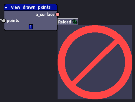
And now your viewer node will look like this when instantiated:
And like this after we execute it:
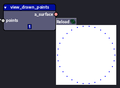
The visualization that appears beside the viewer node is called an in-graph visual, side visual or in-graph surface. Note that the in-graph visual has a button on top that says Reload. As expected, clicking that button causes the node to execute so the visualization is updated. Of course, in order for the node to be executed, the upstream nodes from it are executed as well, so it receives up-to-date inputs.
That's it! At this point, you should be able to test the node pack you created with your get_circle and view_drawn_points nodes.
The alternative way to indicate that your node has a visual to be display beside it is to add a small function in your script called (or aliased as) get_sideviz_from_output. The function must receive a single argument, which is the output of the node, and return the visual data it gets from it (which in our case is a surface). The body of the function can be anything you need to do in order to get the surface from the output of the node that it receives.
Since in our case, the node's output itself is the surface we want to use, that function just needs to return the very argument it receives. Instead of changing the return annotation of our node, we could then just add this line of code to the end of the script and it would have the same effect:
get_sideviz_from_output = lambda node_output: node_outputNote that we arbitrarily decided to call the parameter of our (lambda) function node_output, but you can call it whatever you want. As long as it receives a single argument and returns the surface, it is fine.
When you use the first way (adding/editing the return annotation), Nodezator actually creates this function for you automatically.
Regardless of the method you use to indicate to Nodezator the existence and location of your surface, you might have asked yourself why we need to tell Nodezator where specifically to grab the in-graph surface from the node's output. That is, if there's only one surface, why provide a function to grab it instead of just using a flag that says the output itself is the surface we want? There are 02 answers to that. First, your surface might be nested within the output if you want. In other words, we don't want to impose how your function should work, this is for you to decide. As always, Nodezator tries to get out of your way as much as possible. The second and final reason is that, as we'll see in the next section, the output of the node might contain yet another surface of interest, so we do have to reference each specific surface.
As with any application, the more graphics you display on the screen, the more the performance of the app is impacted. For most cases, the method we described before to provide a surface to be displayed in-graph is more than enough and will result in no harm to the performance, even if you use many viewer nodes like that.
However, what if you wanted to use Nodezator to edit 4K or 8K images, or any kind of data whose visualization resulted in a excessively large surface? In such cases, rather than showing the full visualization in the graph, you may instead want to show a smaller preview, but still provide the full visualization (the larger surface) so that Nodezator can show it in a surface viewer that is invoked when the user clicks the in-graph surface.
This way, you don't need to worry about the size of the surfaces your viewer nodes return. When you create a surface within your node, you just need to ensure it fits a maximum size arbitrarily defined by you and, if the surface is larger than that size, you create a downsized copy of it (probably using the smoothscale() or scale() function from pygame-ce's pygame.transform module). If the surface is smaller than that, you can use it as-is for the in-graph visualization.
Just like the visual data to be displayed beside the node is called in-graph visual, we call this visual data to be visualized in a special viewer full visual or full surface (when it is a surface). We also call it loop data sometimes, since it is data shown in a visualization loop. It just happens that in our demonstration here such data is a surface, but it can be of other types as well, as we'll see in the next section.
As we did previously, before showing how to tell Nodezator that our node provides visual data to be displayed in a dedicated viewer, we'll start by showing a node definition in which the node wasn't turned into a viewer node yet. Here's the definition of a viewer node that receives an image object from the Pillow library in order to visualize it:
### third-party imports

## pygame

from pygame import Surface

from pygame.math import Vector2

from pygame.image import frombytes as surface_from_bytes

from pygame.transform import smoothscale as smoothscale_surface


## Pillow
from PIL.Image import Image


### 2D vector representing origin
ORIGIN = Vector2()


### main callable

def view_image(

    image: Image,
    max_preview_size: 'natural_number' = 600,

) -> [

    {'name': 'full_surface', 'type': Surface},
    {'name': 'preview_surface', 'type': Surface},

]:
    """Return dict with pygame-ce surfaces representing given image.

    Parameters
    ==========
    image
        Pillow image from which to create surfaces.
    max_preview_size
        maximum diagonal length of the preview surface. Must be >= 0.
        If 0, just use the full surface.
    """

    ### obtain surface from pillow image

    mode = image.mode
    size = image.size
    data = image.tobytes()

    full_surface = surface_from_bytes(data, size, mode)

    ### if the max preview size is 0, it means the preview doesn't need
    ### to be below a specific size, so we can use the full surface
    ### as the preview

    if not max_preview_size:

        preview_surface = full_surface

        return {
            'full_surface': full_surface,
            'preview_surface': preview_surface,
        }

    ### otherwise, we must create a preview surface within the allowed size,
    ### if the full surface surpasses such allowed size

    ## obtain the bottom right coordinate of the image, which is
    ## equivalent to its size
    bottomright = full_surface.get_size()

    ## use the bottom right to calculate its diagonal length
    diagonal_length = ORIGIN.distance_to(bottomright)

    ## if the diagonal length of the full surface is higher than the
    ## maximum allowed size, we create a new smaller surface within
    ## the allowed size to use as the preview

    if diagonal_length > max_preview_size:

        size_proportion = max_preview_size / diagonal_length
        new_size = ORIGIN.lerp(bottomright, size_proportion)

        preview_surface = smoothscale_surface(full_surface, new_size)


    ### otherwise, just alias the full surface as the preview surface;
    ###
    ### that is, since the full surface didn't need to be downscaled,
    ### it means it is small enough to be used as an in-graph visual
    ### already

    else:
        preview_surface = full_surface

    ### finally, return a dict containing both surfaces;
    ###
    ### you can return the surfaces in any way you want, inside a list,
    ### inside a tuple or a dictionary, etc.; the format isn't important,
    ### because we specify functions further below in the script to fetch
    ### them for us regardless of where we placed them anyway

    return {
        'full_surface': full_surface,
        'preview_surface': preview_surface,
    }


### alias the function defining the node as main_callable
main_callable = view_image
For now, the definition above just describes a regular node. Again, the special return annotation used by this node has many uses and will be properly presented in a section of a future chapter. Here it doesn't have 'viz' keys, so it is just being used to indicate that this function will return 02 outputs, one named preview_surface and the other full_surface. When this kind of return annotation is used and lists more than 01 output, it means the function must return a dictionary containing the outputs and the names will be used as keys to hold the respective outputs. In other words, this regular node returns a dictionary with a 'preview_surface' and a 'full_surface' key. Now let's see how to turn it into a viewer node.
Just like in the previous section, there are also 02 ways to tell Nodezator that you are providing visual data that is meant to appear in a specialized viewer instead of in the graph itself. They are very similar to the ways shown in the previous section, so pay close attention to the nomenclature.
The first way is by adding/editing the return annotation like this:
{'name': 'full_surface', 'type': Surface, 'viz': 'loop'},
{'name': 'preview_surface', 'type': Surface, 'viz': 'side'},
In other words, we just added the 'viz' key to the outputs used for the in-graph visual and the loop data. The output meant to be used as the in-graph visual, as we saw in the previous section, must have the value 'side' assigned to its 'viz' key. The output meant to be used as the loop data/full visual must have the value 'loop' assigned to its 'viz' key. Again, the 'type' keys are optional and the 'name' keys can have any names you want, as long as it is a valid Python identifier. The outputs can also be in any order you want.
Also, bear in mind that if your node provides loop data/a full visual, it is mandatory that it also provides an side/in-graph visual, like we did here, providing both. Otherwise, Nodezator won't acknowledge the existence of your node as a viewer node.
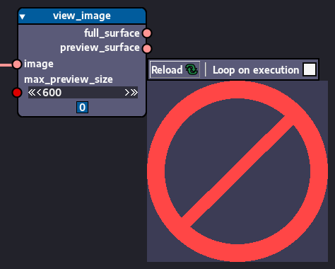
And now this viewer node will look like this when instantiated:
And like this after we execute it:
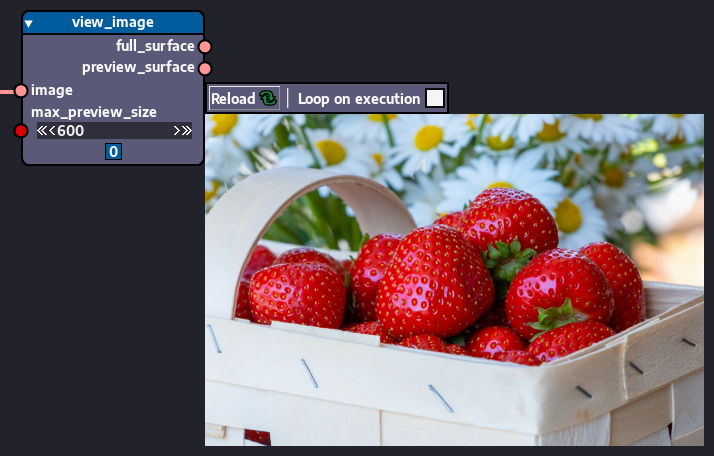
Original strawberry basket image by NickyPe can be found here.
Clicking the in-graph surface showing the strawberry basket in the image above will cause the full surface to be shown using a special surface viewer provided by Nodezator. This viewer has other features as well, like allowing the user to scroll the image using the keyboard or to drag the image around using the mouse.
Note that, in addition to the Reload button, the viewer node now also has a check button labeled Loop on execution. If the check button is marked, whenever the node is executed the app will also enter the loop of the surface viewer. You'll probably leave this button unmarked most of the time, since the in-graph visual will likely be enough.
However, whenever you are fine-tuning the inputs in your graph to obtain a more accurate visualization, you'll probably leave the button marked so that you can inspect the full visual right away, instead of having to click the in-graph visual to access the full view. We'll also demonstrate in a future chapter how to provide a custom visualization loop for your viewer node, in which case leaving this button marked may be useful as well, so you can run your custom visualization when the node is executed.
Another benefit of limiting the size of the surface displayed in the graph is that it makes it easier to organize your graph. That is, when your viewer node can create an in-graph surface of arbitrary size, such surface could end up too large and overlap with neighboring nodes. There's no need to worry if this happens, though, because in-graph visualizations are always drawn behind everything else in the graph, in order to avoid hiding other nodes. However, this is still a undesirable situation, because the other nodes would appear in front of the in-graph visual and you'd have to move the nodes out of the way every time this overlap occurs. Even worse, if the graph is large and has many nodes, you might end up having to move other nodes as well along the graph to make extra space. This is why it is extra useful to use smaller previews for in-graph visuals, instead of full visuals.
As for the second and final way to define a viewer node like this one, you just need to create another function called (or aliased as) get_loopviz_from_output, in addition to your existing get_sideviz_from_output function. This get_loopviz_from_output also receives a single input, which is the output of the node and must return the surface that Nodezator will display whenever the user clicks the in-graph visual.
get_sideviz_from_output = lambda node_output: node_output['preview_surface']
get_loopviz_from_output = lambda node_output: node_output['full_surface']
Again, providing the new get_loopviz_from_output callable requires that a get_sideviz_from_output callable exist as well, in order for Nodezator to acknowledge the existence of your node as a viewer node.
The data used as the side visual data or the loop data doesn't need to be a pygame-ce surface. You can use strings as well. For instance, if you use a string as a side visual, Nodezator will automatically render the text for you and display it like this after the node is executed:
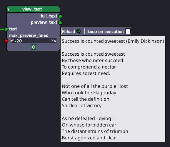
If a string is provided as the loop data, it will be displayed in a text viewer. In other words, just like you can use a smaller surface as the side visual and a full-sized surface as the loop data, you can also display a smaller portion of a text in the graph as a side visual and visualize the full text in a dedicated viewer.
There is actually a custom format that you can use as well. If instead of a string, you provide a dictionary like the one below...
{
    'hint': 'text',
    'data': 'Your text here'
}
...the text in the data key will also be rendered like in the previous image shown.
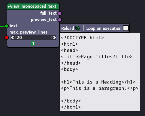
This format can be used to specified different kinds of text so they are rendered differently. For instance, if instead of 'text', the value of the 'hint' key is 'monospaced_text', it will be rendered with a monospaced font, like in the HTML text visualized in the image below:
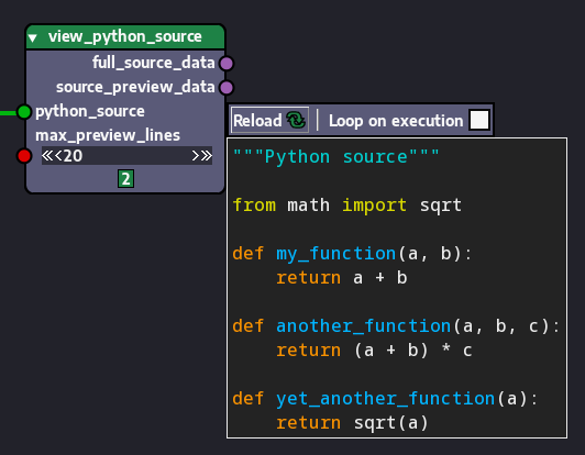
If instead of 'text', the value of the 'hint' key is 'python_source', it will be rendered with a monospaced font and syntax-highlighted as Python code, like the Python code visualized in the image below:
The table below summarizes the values of the 'hint' key that can be used and how the text will be rendered as a result:
| Value of "hint" key | Rendered text |
|---|---|
| "text" | text rendered with variable-width font |
| "monospaced_text" | text rendered with monospaced font |
| "python_source" | text rendered with monospaced font and Python syntax highlighting |
If you use a dict like the ones shown or a string as the loop data, Nodezator will use a text viewer to display the text you provided as the loop data, instead of a surface viewer. Just like we do with surfaces, you can use small texts or a smaller portion of a large text as the in-graph visual data and the full text as the loop data.
Because some viewer nodes are too general, Nodezator comes with a few of them available by default. This way users don't have to copy the same viewer nodes again and again every time they create a new node pack.
Since we have a dedicated chapter on nodes and other objects available by default in Nodezator, we list such general viewer nodes there.
Note that a viewer node that only provides an in-graph visual is not necessarily inferior to one that also provides a full visual. As we said earlier, the full visual is just an additional resource that can be useful when you need to display visuals that are too large (or, as we'll see in other chapters, need to be customized, animated or have additional controls). If you don't need those things and the visuals you produce are not super large images, then you are probably better off just displaying the visuals in-graph.
For instance, if you are working with pixel art (still images), you'll probably only create tiny/small images. If you are only generating static visualizations with matplotlib for a paper, the visuals created won't probably get so large.
Well, in the end, it is up to you which combination of visual features you think you'll need.
As you already know, when a node is in callable mode, a reference to its main callable is passed only the graph. When this is the case, Nodezator has no control over the execution of the node. Because of that Nodezator also cannot store the in-graph visual and the loop data, so the image beside the node cannot be updated, and its stored loop data cannot be updated as well. In fact, that wouldn't even make sense if you think about it. In callable mode, the node represents its behaviour, not a call with its inputs and outputs. It represents an action, that is, the action of grabing inputs and producing outputs (including the visuals). So it can in fact be executed many times along the graph, resulting in varied inputs and outputs. In other words, the action itself (the main callable being passed along) has no particular association with any visualization/outputs produced. That's why, like any other viewer node, simpler viewer nodes like the ones shown in this chapter, that is, viewer nodes that produce in-graph visual and loop data (or just in-graph visuals) have the in-graph visual taken away from them when they are in callable mode.
This is not a bad thing, it is just something that is worth mentioning so that you are not caught by surprise.
In later chapters we'll discover even more ways to provide visualizations with viewer nodes.