Table of contents > Appendix: Recipes
This appendix contains recipes for performing common tasks in a smart/efficient way.
As presented in the chapter on defining your first node, nodes have different modes.
The callable mode in particular can be used to achieve complex tasks with fewer nodes. In other words, nodes in callable mode can simplify your graph a lot while still providing power and versatility. We'll present a tiny example so you can see this in practice. Look at the graph in the image below, where multiple a+b operation nodes are used to add values together:
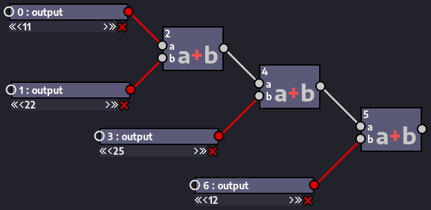
For now the graph is relatively small, but every time you need to add another value, you have to duplicate the operation node and so the graph will gradually become larger and larger.
If you use the a+b node in callable mode, though (by right-clicking it and, inside the Change mode to submenu, picking callable), you would only need a single one. Then you can use it in conjuntion with a functools.reduce() standard library node and a tuple_from_args snippet node to add as many values as you want without having to create several instances of the operator node. The tuple_from_args node is used to gather all values to be added into a single collection (in this case a tuple). Then we pass a reference to the a+b operation as the first argument of functools.reduce() and the collection as the second argument. Here's an alternative version of the graph in the previous image, but using the a+b node in callable mode with the other nodes we just described:
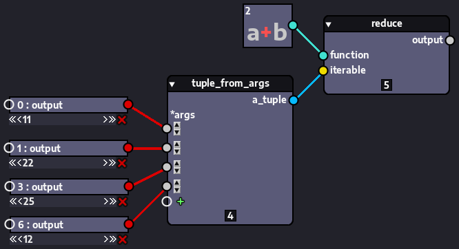
In other words, with just these 03 nodes (a+b, tuple_from_args and functools.reduce()) we can add as many values as we want! In the first version of this graph, if we wanted to add 10 more values, we would need at least 20 more nodes (one node with each new value and another a+b node). In this new version, we'd just need 10 more nodes, which would be the values we'd add to the tuple_from_args node.
You can use this to repeat many different kinds of operations at once. For instance, instead of a+b, you could have used an a*b operation node so all the values would be multiplied.
This is just a tiny example of how the callable mode can be used to achieve complex tasks with a very simple graph.
This section presents a few nodes available by default that can be used alone or in combination to perform many common tasks.
You don't need to define a new node every time you want to grab a value/callable from another module. Nodezator has the importlib.import_module() function available as a standard library node. You can use this node in conjunction with other nodes available by default to grab objects from a module and just pass them along to other nodes or, if it is callable, to execute them.
For instance, a lot of programming problems require the usage of mathematical constants. You can grab them from the math like this:
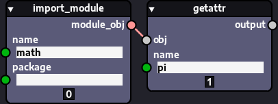
That is, with import_module() you grab the math module and with getattr(), available in Nodezator as a built-in node, you grab the pi attribute from the math module.
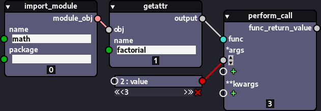
You can also grab a callable object using the same nodes, and execute it using the perform_call snippet node. This node just executes a given callable with given arguments and returns the return-value of the call. The node's source is roughly equivalent to this:
def perform_call(func, *args, **kwargs):
    return func(*args, **kwargs)
Here's how you'd use it in conjunction with importlib.import_module() and getattr() to grab and execute the math.factorial() function:
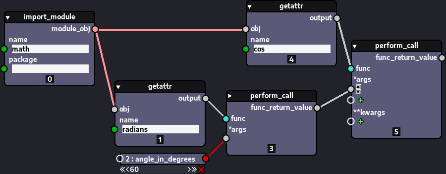
Of course, you can grab as many objects as you want from the imported module. Here we grab a function to convert an angle from degrees to radians and another function to obtain the cosine of the converted angle:
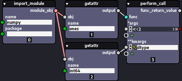
And here we create an array of integers with the numpy library:
Whenever using import_module to import from a third-party library, remember to make sure that library is installed in the Python instance running Nodezator.
The few graphs shown above could be further simplified by using the perform_attr_call node, which you can find in the Encapsulations > perform_attr_call command from the popup menu. This node just encapsulates the behaviour of the getattr and perform_call nodes. It is available by default in Nodezator because grabbing a method or other callable from an attribute in order to execute it is a very common task.
Frequently, we may find ourselves in the need of some small temporary custom code or maybe we just want to experiment with some ideas before we create a new node for some specific purpose. Whenever one of such scenarios arise you can use the namespace_from_exec() node. It allows you to write and execute custom Python code. You can pass it data via keyword arguments and the new names and respective values defined in that code are returned from the node as a dictionary.
Here's a small example of how it can be used:
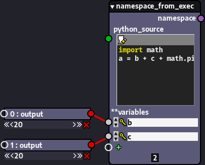
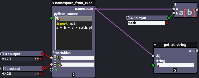
The namespace dictionary returned has all the names defined/referenced in the code:
{'b': 20, 'c': 20, 'math': , 'a': 43.1415926535898} You can grab any or many of such values using nodes like the a[b] operation node or the get_at_string snippet node (which works the same way as a[b], but has a StringEntry widget attached for convenience):
As you may already know, Nodezator provides some viewer nodes by default to visualize pygame-ce surfaces or text.
Although users can also create their own custom viewer nodes, sometimes what they need to visualize can be easily converted into or represented as an image. When this is the case, rather than creating a custom viewer node by themselves, it may actually be better to just convert the data into a pygame-ce surface (or create a regular node to do so). Then, the user can pass the created surface to the view_surface node that is provided by default in Nodezator.
By doing this, your operations will be even more modular and you'll avoid some extra steps that you would otherwise need to tackle yourself if you had to define a custom viewer node, like checking whether a scaled down version of the surface is needed (in order to use it as a preview), and actually creating such extra surface, etc. (although such steps are relatively simple as well).
It is usually straightforward to convert some sort of data into a pygame-ce surface. Below we demonstrate how to convert a Pillow image into a pygame-ce surface using pygame-ce's pygame.image.frombytes:
mode = image.mode
size = image.size
data = image.tobytes()

surface = frombytes(data, size, mode)
Code adapted from this stackoverflow answer.
And below, using the same function, we convert a matplotlib figure:
canvas = figure.canvas
canvas.draw()

raw_data = canvas.tostring_rgb()
size = canvas.get_width_height()

surface = frombytes(raw_data, size, 'RGB')
Code adapted from several sources, including this stackoverflow answer.
This frombytes function is available by default in Nodezator as the surf_from_bytes node, which you can access via the pygame-ce > pygame.image > surf_from_bytes command in the popup menu.
The image below illustrates how a Pillow image could be converted into a surface that would then be visualized with the view_surface. A preview of the surface would appear beside the viewer node and if that preview is clicked, the surface is displayed in full size in a surface viewer.
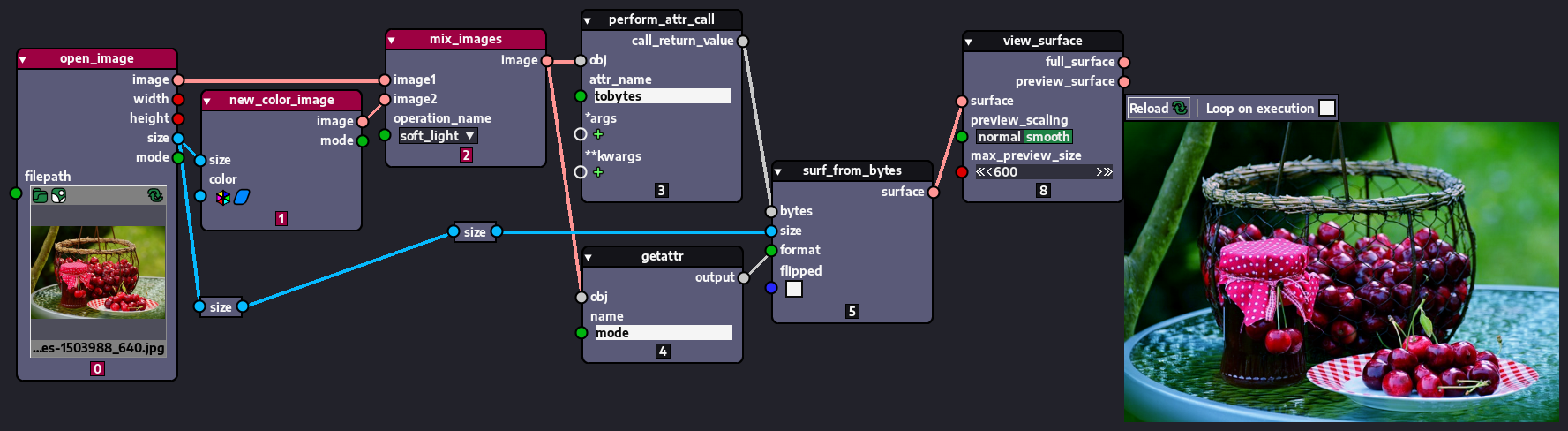
Original cherries image by congerdesign can be found here.
Note that in the case of Pillow images, we didn't even need to create a custom node to convert a Pillow image into a pygame-ce surface. In the graph shown in the image above, we load an image from the disk as a Pillow image, mix it with another Pillow image filled with a single color and mix the 02 images together using a soft light operation. The resulting Pillow image is then converted into a pygame-ce surface and displayed in the view_surface node.
When working with other libraries you might have to create a custom node to produce the needed data to feed into the surf_from_bytes node. The reason nodes that automatically convert objects from various libraries like matplotlib and others aren't available by default in Nodezator is because they are too specialized. That is, although they would be very handy, there are innumerable Python libraries available, all with their own specific data formats. Thus, we would never be able to offer sufficient default nodes to target all of them. As a result, Nodezator only offers the most basic nodes. Additionally, usage of such specialized nodes depend on user choice and needs so, again, it is better that the users decide for themselves which nodes to create and use as they see fit. Last but not least, even simple operations like those may have nuances, so again it is better that users decide for themselves how they want their nodes to be defined and that they create them with the needed parameters and return value.
Another useful function that can be used to convert data into pygame-ce surfaces is pygame.image.load, which is available by default in Nodezator as the load_image_as_surf that can be found in the pygame-ce > pygame.image > load_image_as_surf command from the popup menu. Though this function is usually used to load image files from the disk by passing the image's path to it, you can also pass a io.BytesIO object containing the bytes representing the image. In some cases, depending on the library with which you are treating your BytesIO object, you'll have to call bytes_io_obj.seek(0) before passing the BytesIO object to the load_image_as_surf node.
For instance, if you want to convert an SVG image into a surface, you can use the cairosvg library like this:
from io import BytesIO

from cairosvg import svg2png

new_bites = svg2png(url = 'path_to_file.svg')
bytes_io_obj = BytesIO(new_bites)

surface = pygame.image.load(bytes_io_obj)
Code adapted from this stackoverflow answer.
However, if you wanted to use the sympy library to convert a rendered math formula described in LaTeX markup into a surface, you'd have to call .seek(0) on the BytesIO object, like this:
from io import BytesIO

from sympy import preview

bytes_io_obj = BytesIO()
preview(your_latex_markup, output='png', viewer='BytesIO', outputbuffer=bytes_io_obj)

bytes_io_obj.seek(0) # if you don't do this, the call to pygame.image.load
                     # below will raise an error

surface = pygame.image.load(bytes_io_obj)
Code adapted from this stackoverflow answer which, curiously, also demonstrates how to obtain a surface from a Pillow image using a BytesIO object.
Since sympy uses the LaTeX software internally and related CLI utilities or the matplotlib library for rendering, you'll also need to install one of those in your system for the call to sympy.preview() to work.
In addition to using the load_image_as_surf node, you can also use the surf_from_image_path node from the popup menu command pygame-ce > Encapsulations > surf_from_image_path, that uses pygame.image.load internally, but can also make an extra call to Surface.convert or Surface.convert_alpha. This is usually not needed though, because it just makes it quicker to blit the surface on the screen, which isn't that useful if you only plan on visualizing the surface.
Regardless of how you obtain your surfaces, you can save them back on disk as an image file using pygame.image.save, which is available by default in Nodezator as the save_surf_to_file node found in the pygame-ce > pygame.image > save_surf_to_file command of the popup menu.
Of course, not all data can be represented as a still image. Or perhaps, users may want to add even more parameters to their viewer nodes or add other features. In such cases users are indeed encouraged to define their own custom viewer node(s).